[1]:
import pandas as pd
import numpy as np
import time
import normet as nm
import matplotlib.pyplot as plt
import matplotlib
from pylab import savefig
[2]:
df1=pd.read_csv(r'data/MY1_data.csv',parse_dates=['date'],index_col='date')
[3]:
df1
[3]:
| O3 | NO | NO2 | NOXasNO2 | SO2 | CO | PM10 | NV10 | V10 | PM2.5 | ... | d2m | t2m | blh | sp | ssrd | tcc | tp | rh2m | lat | lon | |
|---|---|---|---|---|---|---|---|---|---|---|---|---|---|---|---|---|---|---|---|---|---|
| date | |||||||||||||||||||||
| 2020-01-01 00:00:00 | 1.72961 | 78.38595 | 45.77784 | 165.96796 | 4.75424 | NaN | 69.0 | 60.0 | 9.0 | 58.1 | ... | 277.183465 | 278.394725 | 384.209053 | 102252.303312 | -1.164153e-10 | 0.650958 | 0.000008 | 91.884130 | 51.52253 | -0.154611 |
| 2020-01-01 01:00:00 | 1.92918 | 88.61587 | 52.64325 | 188.51903 | 4.84394 | 0.397528 | 45.0 | 38.4 | 6.6 | 43.2 | ... | 276.695430 | 277.772899 | 353.220263 | 102211.168636 | -1.164153e-10 | 0.603699 | 0.000002 | 92.715877 | 51.52253 | -0.154611 |
| 2020-01-01 02:00:00 | 1.99570 | 70.02935 | 44.76870 | 152.14554 | 3.09474 | 0.346417 | 46.2 | 39.1 | 7.1 | 43.0 | ... | 276.505662 | 277.463419 | 255.911846 | 102174.855967 | -1.164153e-10 | 0.710378 | 0.000005 | 93.485560 | 51.52253 | -0.154611 |
| 2020-01-01 03:00:00 | 2.04559 | 67.58589 | 40.20699 | 143.83725 | 2.96019 | 0.335059 | 45.1 | 38.8 | 6.3 | 42.8 | ... | 276.412816 | 277.305813 | 191.375560 | 102166.786485 | -1.164153e-10 | 0.837765 | 0.000005 | 93.906363 | 51.52253 | -0.154611 |
| 2020-01-01 04:00:00 | 2.99355 | 72.03298 | 47.26010 | 157.70912 | 3.83478 | 0.349257 | 40.8 | 34.2 | 6.6 | 36.8 | ... | 276.553051 | 277.478941 | 151.780210 | 102142.578039 | -1.164153e-10 | 0.819103 | 0.000003 | 93.696878 | 51.52253 | -0.154611 |
| ... | ... | ... | ... | ... | ... | ... | ... | ... | ... | ... | ... | ... | ... | ... | ... | ... | ... | ... | ... | ... | ... |
| 2020-12-31 19:00:00 | 20.70539 | 12.46950 | 30.47461 | 49.59424 | 1.12164 | 0.129904 | 13.9 | 11.8 | 2.1 | 11.7 | ... | 272.197565 | 273.557442 | 476.945688 | 99902.506413 | -5.820766e-11 | 0.918149 | 0.000000 | 90.582979 | 51.52253 | -0.154611 |
| 2020-12-31 20:00:00 | 24.14797 | 9.65279 | 26.51175 | 41.31249 | 1.12164 | 0.094180 | 14.6 | 11.3 | 3.3 | 11.0 | ... | 272.171041 | 273.629146 | 486.665851 | 99947.625909 | -5.820766e-11 | 0.839639 | 0.000000 | 89.939908 | 51.52253 | -0.154611 |
| 2020-12-31 21:00:00 | 25.69464 | 12.46950 | 28.45232 | 47.57196 | 1.36199 | 0.087685 | 16.6 | 13.0 | 3.6 | 15.3 | ... | 272.087408 | 273.470592 | 489.355002 | 100000.215520 | -5.820766e-11 | 0.739354 | 0.000000 | 90.422188 | 51.52253 | -0.154611 |
| 2020-12-31 22:00:00 | 26.39313 | 6.45629 | 25.05721 | 34.95672 | 0.88129 | 0.084437 | 19.1 | 16.0 | 3.1 | 17.1 | ... | 272.235319 | 272.926062 | 40.714872 | 100042.844978 | -5.820766e-11 | 0.643753 | 0.000000 | 95.088677 | 51.52253 | -0.154611 |
| 2020-12-31 23:00:00 | 27.93980 | 6.61453 | 22.07004 | 32.21218 | 0.88129 | 0.087685 | 17.6 | 13.2 | 4.4 | 15.2 | ... | 272.020979 | 272.681367 | 55.617254 | 100053.601944 | -5.820766e-11 | 0.549403 | 0.000000 | 95.290673 | 51.52253 | -0.154611 |
8784 rows × 65 columns
AutoML-based weather normalisation
[4]:
df1a=nm.prepare_data(df1, value='PM2.5', feature_names=['u10', 'v10', 'd2m', 't2m',
       'blh', 'sp', 'ssrd', 'tcc', 'tp', 'rh2m'], split_method='random',  fraction=0.75, seed=7654321)
[5]:
model_config = {
        'time_budget': 90,                     # Total running time in seconds
        'metric': 'r2',                        # Primary metric for regression, 'mae', 'mse', 'r2', 'mape',...
        'estimator_list': ["lgbm"],            # List of ML learners: "lgbm", "rf", "xgboost", "extra_tree", "xgb_limitdepth"
    }
[6]:
model1=nm.train_model(df1a,variables=['u10', 'v10', 'd2m', 't2m',
       'blh', 'sp', 'ssrd', 'tcc', 'tp', 'rh2m','date_unix', 'day_julian', 'weekday',
       'hour'],model_config =model_config );
2024-09-24 16:20:23 : Training AutoML...
2024-09-24 16:21:57 : Best model is lgbm with best model parameters of {'n_estimators': 4779, 'num_leaves': 37, 'min_child_samples': 13, 'learning_rate': 0.05353325544814332, 'log_max_bin': 10, 'colsample_bytree': 0.7006661480744041, 'reg_alpha': 3.4963871783049667, 'reg_lambda': 0.12148015741620988}
[7]:
model1
[7]:
AutoML(append_log=False, auto_augment=True, custom_hp={},
       cv_score_agg_func=None, early_stop=False, ensemble=False,
       estimator_list='auto', eval_method='auto', fit_kwargs_by_estimator={},
       force_cancel=False, free_mem_ratio=0, hpo_method='auto',
       keep_search_state=False, learner_selector='sample', log_file_name='',
       log_training_metric=False, log_type='better', max_iter=None,
       mem_thres=4294967296, metric='auto', metric_constraints=[],
       min_sample_size=10000, mlflow_logging=True, model_history=False,
       n_concurrent_trials=1, n_jobs=-1, n_splits=5, pred_time_limit=inf,
       preserve_checkpoint=True, retrain_full=True, ...)
In a Jupyter environment, please rerun this cell to show the HTML representation or trust the notebook. On GitHub, the HTML representation is unable to render, please try loading this page with nbviewer.org.
AutoML(append_log=False, auto_augment=True, custom_hp={},
       cv_score_agg_func=None, early_stop=False, ensemble=False,
       estimator_list='auto', eval_method='auto', fit_kwargs_by_estimator={},
       force_cancel=False, free_mem_ratio=0, hpo_method='auto',
       keep_search_state=False, learner_selector='sample', log_file_name='',
       log_training_metric=False, log_type='better', max_iter=None,
       mem_thres=4294967296, metric='auto', metric_constraints=[],
       min_sample_size=10000, mlflow_logging=True, model_history=False,
       n_concurrent_trials=1, n_jobs=-1, n_splits=5, pred_time_limit=inf,
       preserve_checkpoint=True, retrain_full=True, ...)
[8]:
best_model = model1.best_estimator
best_config = model1.best_config
print("Best model:", best_model)
print("Best model parameters:", best_config)
model1.best_result
Best model: lgbm
Best model parameters: {'n_estimators': 4779, 'num_leaves': 37, 'min_child_samples': 13, 'learning_rate': 0.05353325544814332, 'log_max_bin': 10, 'colsample_bytree': 0.7006661480744041, 'reg_alpha': 3.4963871783049667, 'reg_lambda': 0.12148015741620988}
[8]:
{'pred_time': 1.9110346438994467e-05,
 'wall_clock_time': 90.33755874633789,
 'metric_for_logging': {'pred_time': 1.9110346438994467e-05},
 'val_loss': 0.12917426813136582,
 'training_iteration': 1,
 'config': {'n_estimators': 4779,
  'num_leaves': 37,
  'min_child_samples': 13,
  'learning_rate': 0.05353325544814332,
  'log_max_bin': 10,
  'colsample_bytree': 0.7006661480744041,
  'reg_alpha': 3.4963871783049667,
  'reg_lambda': 0.12148015741620988},
 'config/n_estimators': 4779,
 'config/num_leaves': 37,
 'config/min_child_samples': 13,
 'config/learning_rate': 0.05353325544814332,
 'config/log_max_bin': 10,
 'config/colsample_bytree': 0.7006661480744041,
 'config/reg_alpha': 3.4963871783049667,
 'config/reg_lambda': 0.12148015741620988,
 'experiment_tag': 'exp',
 'time_total_s': 9.342859029769897}
[9]:
model1.feature_importances_
[9]:
array([ 993, 6549, 6934, 5345, 5295, 6633, 6315, 4237, 6126, 3377, 6176,
       4652, 1062, 3878], dtype=int32)
[10]:
model1.feature_names_in_
[10]:
['weekday',
 'u10',
 'v10',
 'd2m',
 't2m',
 'blh',
 'sp',
 'ssrd',
 'tcc',
 'tp',
 'rh2m',
 'date_unix',
 'day_julian',
 'hour']
[11]:
model_config = {
        'time_budget': 90,
        #'max_models': 10,              # Maximum number of models to train
        #'max_mem_size': '12g',         # Maximum memory size for H2O
        'estimator_list': ['GBM'],     # List of algorithms to use in AutoML
    }
[12]:
model2=nm.train_model(df1a,automl_pkg='h2o',variables=['u10', 'v10', 'd2m', 't2m',
       'blh', 'sp', 'ssrd', 'tcc', 'tp', 'rh2m','date_unix', 'day_julian', 'weekday',
       'hour'],model_config=model_config);
H2O is not running. Starting H2O...
Checking whether there is an H2O instance running at http://localhost:54321. connected.
| H2O_cluster_uptime: | 3 hours 59 mins |
| H2O_cluster_timezone: | Europe/London |
| H2O_data_parsing_timezone: | UTC |
| H2O_cluster_version: | 3.46.0.5 |
| H2O_cluster_version_age: | 26 days |
| H2O_cluster_name: | H2O_from_python_n94921cs_5qrqdn |
| H2O_cluster_total_nodes: | 1 |
| H2O_cluster_free_memory: | 7.572 Gb |
| H2O_cluster_total_cores: | 8 |
| H2O_cluster_allowed_cores: | 1 |
| H2O_cluster_status: | locked, healthy |
| H2O_connection_url: | http://localhost:54321 |
| H2O_connection_proxy: | {"http": null, "https": null} |
| H2O_internal_security: | False |
| Python_version: | 3.12.2 final |
2024-09-24 16:21:58: Training AutoML...
2024-09-24 16:22:42: Best model obtained! - GBM_grid_1_AutoML_4_20240924_162158_model_2
[13]:
model2
[13]:
Model Details
=============
H2OGradientBoostingEstimator : Gradient Boosting Machine
Model Key: GBM_grid_1_AutoML_4_20240924_162158_model_2
| number_of_trees | number_of_internal_trees | model_size_in_bytes | min_depth | max_depth | mean_depth | min_leaves | max_leaves | mean_leaves | |
|---|---|---|---|---|---|---|---|---|---|
| 69.0 | 69.0 | 1189276.0 | 13.0 | 13.0 | 13.0 | 625.0 | 1942.0 | 1369.2754 |
ModelMetricsRegression: gbm
** Reported on train data. **

MSE: 0.011242541344013361
RMSE: 0.10603085090676846
MAE: 0.07893400538333294
RMSLE: NaN
Mean Residual Deviance: 0.011242541344013361
ModelMetricsRegression: gbm
** Reported on cross-validation data. **

MSE: 8.126360199772725
RMSE: 2.850677147586644
MAE: 1.9222905950632483
RMSLE: NaN
Mean Residual Deviance: 8.126360199772725
| mean | sd | cv_1_valid | cv_2_valid | cv_3_valid | cv_4_valid | cv_5_valid | |
|---|---|---|---|---|---|---|---|
| aic | nan | 0.0 | nan | nan | nan | nan | nan |
| loglikelihood | nan | 0.0 | nan | nan | nan | nan | nan |
| mae | 1.9222906 | 0.0324555 | 1.9084675 | 1.9052794 | 1.888859 | 1.9710108 | 1.9378362 |
| mean_residual_deviance | 8.12636 | 0.6548642 | 8.182448 | 7.1749625 | 7.8459816 | 8.850865 | 8.577542 |
| mse | 8.12636 | 0.6548642 | 8.182448 | 7.1749625 | 7.8459816 | 8.850865 | 8.577542 |
| r2 | 0.8793102 | 0.0095628 | 0.8805432 | 0.8902119 | 0.8867002 | 0.8692322 | 0.8698634 |
| residual_deviance | 8.12636 | 0.6548642 | 8.182448 | 7.1749625 | 7.8459816 | 8.850865 | 8.577542 |
| rmse | 2.8487926 | 0.1158737 | 2.860498 | 2.678612 | 2.801068 | 2.9750404 | 2.928744 |
| rmsle | nan | 0.0 | nan | nan | nan | nan | nan |
| timestamp | duration | number_of_trees | training_rmse | training_mae | training_deviance | |
|---|---|---|---|---|---|---|
| 2024-09-24 16:22:28 | 7.661 sec | 0.0 | 8.2062346 | 5.4746640 | 67.3422868 | |
| 2024-09-24 16:22:28 | 7.723 sec | 5.0 | 5.0442433 | 3.4151840 | 25.4443903 | |
| 2024-09-24 16:22:28 | 7.779 sec | 10.0 | 3.1914116 | 2.2053144 | 10.1851080 | |
| 2024-09-24 16:22:28 | 7.835 sec | 15.0 | 2.0162629 | 1.4358716 | 4.0653160 | |
| 2024-09-24 16:22:28 | 7.892 sec | 20.0 | 1.3258726 | 0.9765391 | 1.7579382 | |
| 2024-09-24 16:22:28 | 7.957 sec | 25.0 | 0.8801164 | 0.6675258 | 0.7746049 | |
| 2024-09-24 16:22:28 | 8.014 sec | 30.0 | 0.6213492 | 0.4796348 | 0.3860749 | |
| 2024-09-24 16:22:28 | 8.067 sec | 35.0 | 0.4578002 | 0.3572500 | 0.2095810 | |
| 2024-09-24 16:22:28 | 8.132 sec | 40.0 | 0.3379802 | 0.2647451 | 0.1142306 | |
| 2024-09-24 16:22:28 | 8.191 sec | 45.0 | 0.2648459 | 0.2051404 | 0.0701433 | |
| 2024-09-24 16:22:28 | 8.251 sec | 50.0 | 0.2069501 | 0.1595394 | 0.0428284 | |
| 2024-09-24 16:22:28 | 8.305 sec | 55.0 | 0.1663724 | 0.1275311 | 0.0276798 | |
| 2024-09-24 16:22:28 | 8.354 sec | 60.0 | 0.1397592 | 0.1064105 | 0.0195326 | |
| 2024-09-24 16:22:28 | 8.408 sec | 65.0 | 0.1167263 | 0.0878304 | 0.0136250 | |
| 2024-09-24 16:22:29 | 8.495 sec | 69.0 | 0.1060309 | 0.0789340 | 0.0112425 |
| variable | relative_importance | scaled_importance | percentage |
|---|---|---|---|
| u10 | 251463.8437500 | 1.0 | 0.1484518 |
| blh | 210509.4843750 | 0.8371362 | 0.1242744 |
| d2m | 202005.6875000 | 0.8033190 | 0.1192542 |
| day_julian | 201374.0937500 | 0.8008073 | 0.1188813 |
| sp | 158984.7187500 | 0.6322369 | 0.0938567 |
| date_unix | 130323.0937500 | 0.5182578 | 0.0769363 |
| t2m | 108348.5078125 | 0.4308711 | 0.0639636 |
| v10 | 87987.5078125 | 0.3499012 | 0.0519435 |
| weekday | 81752.5156250 | 0.3251064 | 0.0482626 |
| rh2m | 80490.9296875 | 0.3200895 | 0.0475179 |
| hour | 61422.0507812 | 0.2442580 | 0.0362605 |
| tcc | 57315.1562500 | 0.2279260 | 0.0338360 |
| ssrd | 46235.0937500 | 0.1838638 | 0.0272949 |
| tp | 15695.9404297 | 0.0624183 | 0.0092661 |
[tips]
Use `model.explain()` to inspect the model.
--
Use `h2o.display.toggle_user_tips()` to switch on/off this section.
[14]:
?nm.train_model
Signature:
nm.train_model(
    df,
    value='value',
    automl_pkg='flaml',
    variables=None,
    model_config=None,
    seed=7654321,
    n_cores=None,
    verbose=True,
)
Docstring:
Trains a machine learning model using either FLAML or H2O AutoML.

Parameters:
    df (pandas.DataFrame): Input dataset to train the model.
    value (str): The name of the target column in the dataset. Default is "value".
    automl_pkg (str): The AutoML package to use ("flaml" or "h2o").
    variables (list, optional): List of feature variables to use for training.
    model_config (dict, optional): Configuration settings for the model training.
    seed (int, optional): Random seed for reproducibility. Default is 7654321.
    n_cores (int, optional): Number of CPU cores to use for training. Default is None.
    verbose (bool, optional): Whether to print detailed logs. Default is True.

Returns:
    model: Trained machine learning model with a custom attribute `_model_type` indicating the package used.
File:      ~/anaconda3/envs/normet/lib/python3.12/site-packages/normet/normet.py
Type:      function
[15]:
mod_stats1=nm.modStats(df1a,model1)
[16]:
mod_stats1
[16]:
| n | FAC2 | MB | MGE | NMB | NMGE | RMSE | r | p_level | COE | IOA | R2 | set | |
|---|---|---|---|---|---|---|---|---|---|---|---|---|---|
| 0 | 4780 | 0.987238 | -0.000007 | 0.268328 | -7.437997e-07 | 0.029447 | 0.351283 | 0.999110 | *** | 0.950987 | 0.975494 | 0.998222 | training |
| 1 | 1593 | 0.907721 | 0.090223 | 1.920277 | 9.806910e-03 | 0.208727 | 2.699133 | 0.940890 | *** | 0.650259 | 0.825129 | 0.885274 | testing |
| 2 | 6373 | 0.967362 | 0.022547 | 0.681250 | 2.468418e-03 | 0.074582 | 1.383329 | 0.985535 | *** | 0.875668 | 0.937834 | 0.971279 | all |
[17]:
mod_stats2=nm.modStats(df1a,model2)
[18]:
mod_stats2
[18]:
| n | FAC2 | MB | MGE | NMB | NMGE | RMSE | r | p_level | COE | IOA | R2 | set | |
|---|---|---|---|---|---|---|---|---|---|---|---|---|---|
| 0 | 4780 | 0.994142 | 2.145110e-08 | 0.078934 | 2.354070e-09 | 0.008662 | 0.106031 | 0.999923 | *** | 0.985582 | 0.992791 | 0.999846 | training |
| 1 | 1593 | 0.901444 | 1.458128e-01 | 1.952102 | 1.584932e-02 | 0.212186 | 2.753047 | 0.939557 | *** | 0.644462 | 0.822231 | 0.882767 | testing |
| 2 | 6373 | 0.970971 | 3.644749e-02 | 0.547153 | 3.990205e-03 | 0.059901 | 1.379475 | 0.985645 | *** | 0.900142 | 0.950071 | 0.971496 | all |
[19]:
start_time = time.time()
df_dew1=nm.normalise(df1a,model1,
                           feature_names=['u10', 'v10', 'd2m', 't2m',
       'blh', 'sp', 'ssrd', 'tcc', 'tp', 'rh2m','date_unix', 'day_julian', 'weekday',
       'hour'],
                          variables_resample= ['u10', 'v10', 'd2m', 't2m',
       'blh', 'sp', 'ssrd', 'tcc', 'tp', 'rh2m'],
                          n_samples=1000,aggregate=True)
end_time = time.time()

# 计算执行时间
execution_time = end_time - start_time
print(f"Execution time: {execution_time:.2f} seconds")
2024-09-24 16:22:45: Normalising the dataset in parallel.
2024-09-24 16:22:47: Predicting using trained model in batches.
2024-09-24 16:25:07: Aggregating 1000 predictions...
Execution time: 142.41 seconds
[20]:
start_time = time.time()
df_dew2=nm.normalise(df1a,model2,
                           feature_names=['u10', 'v10', 'd2m', 't2m',
       'blh', 'sp', 'ssrd', 'tcc', 'tp', 'rh2m','date_unix', 'day_julian', 'weekday',
       'hour'],
                          variables_resample= ['u10', 'v10', 'd2m', 't2m',
       'blh', 'sp', 'ssrd', 'tcc', 'tp', 'rh2m'],
                          n_samples=1000,aggregate=True)
end_time = time.time()

# 计算执行时间
execution_time = end_time - start_time
print(f"Execution time: {execution_time:.2f} seconds")
2024-09-24 16:25:08: Normalising the dataset in parallel.
2024-09-24 16:25:09: Predicting using trained model in batches.
2024-09-24 16:29:04: Aggregating 1000 predictions...
Execution time: 236.45 seconds
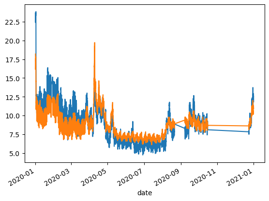
[21]:
fig,ax=plt.subplots()
df_dew1['normalised'].plot()
df_dew2['normalised'].plot()
[21]:
<Axes: xlabel='date'>
[22]:
start_time = time.time()
df_dew3=nm.normalise(df1a,model1,
                           feature_names=['u10', 'v10', 'd2m', 't2m',
       'blh', 'sp', 'ssrd', 'tcc', 'tp', 'rh2m','date_unix', 'day_julian', 'weekday',
       'hour'],
                          variables_resample= ['u10', 'v10', 'd2m', 't2m',
       'blh', 'sp', 'ssrd', 'tcc', 'tp', 'rh2m'],
                          n_samples=1000,aggregate=False)
end_time = time.time()

# 计算执行时间
execution_time = end_time - start_time
print(f"Execution time: {execution_time:.2f} seconds")
2024-09-24 16:29:05: Normalising the dataset in parallel.
2024-09-24 16:29:06: Predicting using trained model in batches.
Execution time: 143.14 seconds
[23]:
df_dew3.head()
[23]:
| date | observed | normalised | seed | |
|---|---|---|---|---|
| 0 | 2020-01-01 00:00:00 | 58.1 | 17.221536 | 979812 |
| 1 | 2020-01-01 01:00:00 | 43.2 | 32.937436 | 979812 |
| 2 | 2020-01-01 02:00:00 | 43.0 | 24.423807 | 979812 |
| 3 | 2020-01-01 03:00:00 | 42.8 | 23.372347 | 979812 |
| 4 | 2020-01-01 04:00:00 | 36.8 | 26.478917 | 979812 |
[24]:
weather_df=df1.reset_index().iloc[0:100][['u10', 'v10', 'd2m', 't2m',
       'blh', 'sp', 'ssrd', 'tcc', 'tp', 'rh2m']]
[25]:
weather_df.head()
[25]:
| u10 | v10 | d2m | t2m | blh | sp | ssrd | tcc | tp | rh2m | |
|---|---|---|---|---|---|---|---|---|---|---|
| 0 | -2.720528 | 1.545010 | 277.183465 | 278.394725 | 384.209053 | 102252.303312 | -1.164153e-10 | 0.650958 | 0.000008 | 91.884130 |
| 1 | -2.308789 | 1.282742 | 276.695430 | 277.772899 | 353.220263 | 102211.168636 | -1.164153e-10 | 0.603699 | 0.000002 | 92.715877 |
| 2 | -2.216471 | 0.758730 | 276.505662 | 277.463419 | 255.911846 | 102174.855967 | -1.164153e-10 | 0.710378 | 0.000005 | 93.485560 |
| 3 | -1.928623 | 0.509013 | 276.412816 | 277.305813 | 191.375560 | 102166.786485 | -1.164153e-10 | 0.837765 | 0.000005 | 93.906363 |
| 4 | -1.700043 | 0.607069 | 276.553051 | 277.478941 | 151.780210 | 102142.578039 | -1.164153e-10 | 0.819103 | 0.000003 | 93.696878 |
[26]:
start_time = time.time()
df_dew2=nm.normalise(df1a, model1, weather_df=weather_df,
                           feature_names=['u10', 'v10', 'd2m', 't2m',
       'blh', 'sp', 'ssrd', 'tcc', 'tp', 'rh2m','date_unix', 'day_julian', 'weekday',
       'hour'],
                          variables_resample= ['u10', 'v10', 'd2m', 't2m',
       'blh', 'sp', 'ssrd', 'tcc', 'tp', 'rh2m'],
                          n_samples=300,aggregate=True)
end_time = time.time()

# 计算执行时间
execution_time = end_time - start_time
print(f"Execution time: {execution_time:.2f} seconds")
2024-09-24 16:31:28: Normalising the dataset in parallel.
2024-09-24 16:31:28: Predicting using trained model in batches.
2024-09-24 16:32:10: Aggregating 300 predictions...
Execution time: 42.37 seconds
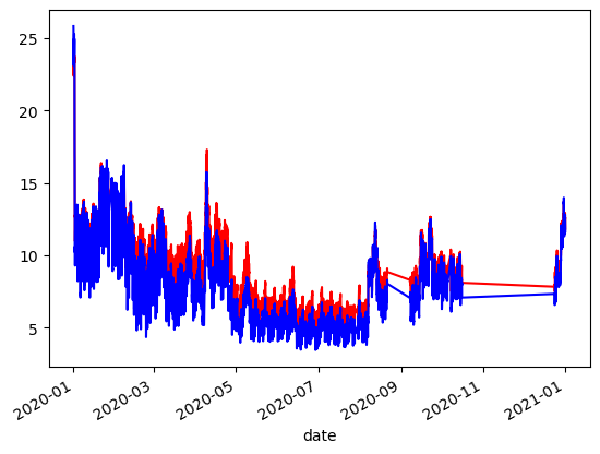
[27]:
df_dew1['normalised'].plot(c='r')
df_dew2['normalised'].plot(c='b')
[27]:
<Axes: xlabel='date'>
[28]:
model_config={
    'time_budget': 60,  # Total running time in seconds
    'metric': 'r2', #
}
[29]:
df1a.columns
[29]:
Index(['rowid', 'd2m', 'blh', 'ssrd', 't2m', 'v10', 'u10', 'sp', 'tp', 'tcc',
       'rh2m', 'date', 'value', 'date_unix', 'day_julian', 'weekday', 'hour',
       'set'],
      dtype='object')
[30]:
df_dew, mod_stats=nm.do_all(df1,value='PM2.5',feature_names=['u10', 'v10', 'd2m', 't2m',
       'blh', 'sp', 'ssrd', 'tcc', 'tp', 'rh2m','date_unix', 'day_julian', 'weekday',
       'hour'],variables_resample=['u10', 'v10', 'd2m', 't2m',
       'blh', 'sp', 'ssrd', 'tcc', 'tp', 'rh2m'],model_config=model_config,n_samples=100)
2024-09-24 16:32:10 : Training AutoML...
2024-09-24 16:33:08 : Best model is lgbm with best model parameters of {'n_estimators': 527, 'num_leaves': 57, 'min_child_samples': 19, 'learning_rate': 0.10029209493914669, 'log_max_bin': 10, 'colsample_bytree': 0.777659907533841, 'reg_alpha': 5.054157418960246, 'reg_lambda': 0.023089272254781048}
2024-09-24 16:33:09: Normalising the dataset in parallel.
2024-09-24 16:33:09: Predicting using trained model in batches.
2024-09-24 16:33:14: Aggregating 100 predictions...
[31]:
df_dew, mod_stats=nm.do_all(df1a,model1,feature_names=['u10', 'v10', 'd2m', 't2m',
       'blh', 'sp', 'ssrd', 'tcc', 'tp', 'rh2m','date_unix', 'day_julian', 'weekday',
       'hour'],variables_resample=['u10', 'v10', 'd2m', 't2m',
       'blh', 'sp', 'ssrd', 'tcc', 'tp', 'rh2m'],model_config=model_config,n_samples=100)
2024-09-24 16:33:15: Normalising the dataset in parallel.
2024-09-24 16:33:15: Predicting using trained model in batches.
2024-09-24 16:33:28: Aggregating 100 predictions...
[32]:
#Resampling from given dataset
df_dew, mod_stats=nm.do_all(df1a,model1,feature_names=['u10', 'v10', 'd2m', 't2m',
       'blh', 'sp', 'ssrd', 'tcc', 'tp', 'rh2m','date_unix', 'day_julian', 'weekday',
       'hour'],variables_resample=['u10', 'v10', 'd2m', 't2m',
       'blh', 'sp', 'ssrd', 'tcc', 'tp', 'rh2m'],weather_df=weather_df,model_config=model_config,n_samples=100)
2024-09-24 16:33:29: Normalising the dataset in parallel.
2024-09-24 16:33:29: Predicting using trained model in batches.
2024-09-24 16:33:42: Aggregating 100 predictions...
[33]:
df_dew, mod_stats=nm.do_all_unc(df1,value='PM2.5',feature_names=['u10', 'v10', 'd2m', 't2m',
       'blh', 'sp', 'ssrd', 'tcc', 'tp', 'rh2m','date_unix', 'day_julian', 'weekday',
       'hour'],variables_resample=['u10', 'v10', 'd2m', 't2m',
       'blh', 'sp', 'ssrd', 'tcc', 'tp', 'rh2m'],n_samples=100,n_models=5)
2024-09-24 16:35:15 : Progress: 20.00% (Model 1/5)... ETA: 6.22 minutes
2024-09-24 16:37:17 : Progress: 40.00% (Model 2/5)... ETA: 5.37 minutes
2024-09-24 16:39:04 : Progress: 60.00% (Model 3/5)... ETA: 3.58 minutes
2024-09-24 16:41:10 : Progress: 80.00% (Model 4/5)... ETA: 1.87 minutes
2024-09-24 16:42:49 : Progress: 100.00% (Model 5/5)... ETA: 0.00 seconds
[34]:
df_dew.head()
[34]:
| observed | normalised_979812 | normalised_378829 | normalised_120727 | normalised_541475 | normalised_488292 | mean | std | median | lower_bound | upper_bound | weighted | |
|---|---|---|---|---|---|---|---|---|---|---|---|---|
| date | ||||||||||||
| 2020-01-01 00:00:00 | 58.1 | 30.252205 | 26.007282 | 21.472511 | 13.609010 | 13.521217 | 20.972445 | 6.655142 | 21.472511 | 13.529996 | 29.827713 | 20.220786 |
| 2020-01-01 01:00:00 | 43.2 | 30.718119 | 22.379913 | 22.043467 | 11.979618 | 14.756184 | 20.375460 | 6.570192 | 22.043467 | 12.257275 | 29.884298 | 18.638353 |
| 2020-01-01 02:00:00 | 43.0 | 30.120009 | 21.627895 | 20.220487 | 13.131916 | 14.394936 | 19.899048 | 6.060521 | 20.220487 | 13.258218 | 29.270797 | 18.202305 |
| 2020-01-01 03:00:00 | 42.8 | 28.591281 | 21.836566 | 22.887696 | 11.813100 | 12.544112 | 19.534551 | 6.435126 | 21.836566 | 11.886201 | 28.020922 | 18.432641 |
| 2020-01-01 04:00:00 | 36.8 | 30.390922 | 21.896232 | 21.653471 | 12.113235 | 12.944652 | 19.799702 | 6.724275 | 21.653471 | 12.196376 | 29.541453 | 18.257228 |
Time series decomposition
[35]:
df_dewca, mod_stats=nm.decom_emi(df1, value='PM2.5',feature_names=['u10', 'v10', 'd2m', 't2m',
       'blh', 'sp', 'ssrd', 'tcc', 'tp', 'rh2m','date_unix', 'day_julian', 'weekday',
       'hour'], split_method = 'random', fraction=0.75, n_samples=300)
2024-09-24 16:42:49 : Training AutoML...
2024-09-24 16:44:15 : Best model is lgbm with best model parameters of {'n_estimators': 4779, 'num_leaves': 37, 'min_child_samples': 13, 'learning_rate': 0.05353325544814332, 'log_max_bin': 10, 'colsample_bytree': 0.7006661480744041, 'reg_alpha': 3.4963871783049667, 'reg_lambda': 0.12148015741620988}
2024-09-24 16:44:15 : Subtracting base...
2024-09-24 16:44:59 : Subtracting date_unix... ETA: 2.93 minutes
2024-09-24 16:45:41 : Subtracting day_julian... ETA: 2.16 minutes
2024-09-24 16:46:27 : Subtracting weekday... ETA: 1.46 minutes
2024-09-24 16:47:12 : Subtracting hour... ETA: 44.25 seconds
[36]:
df_dewca
[36]:
| observed | base | date_unix | day_julian | weekday | hour | deweathered | emi_noise | |
|---|---|---|---|---|---|---|---|---|
| date | ||||||||
| 2020-01-01 00:00:00 | 58.1 | 9.834232 | 18.762883 | 3.617389 | 0.991752 | 0.271323 | 24.320077 | 0.676729 |
| 2020-01-01 01:00:00 | 43.2 | 9.211363 | 19.549169 | 3.381027 | 0.795226 | 0.420953 | 24.200235 | 0.053860 |
| 2020-01-01 02:00:00 | 43.0 | 8.740657 | 18.760258 | 4.192777 | 0.800782 | -0.187559 | 23.149413 | -0.416846 |
| 2020-01-01 03:00:00 | 42.8 | 8.869214 | 18.804496 | 3.959970 | 0.529601 | -0.208110 | 22.797669 | -0.288289 |
| 2020-01-01 04:00:00 | 36.8 | 8.184215 | 19.394484 | 3.038679 | 0.761000 | 0.107604 | 22.328479 | -0.973288 |
| ... | ... | ... | ... | ... | ... | ... | ... | ... |
| 2020-12-31 19:00:00 | 11.7 | 8.621910 | 12.759990 | 0.336607 | -0.046839 | 0.406496 | 12.920661 | -0.535593 |
| 2020-12-31 20:00:00 | 11.0 | 8.749583 | 12.430059 | 0.528524 | -0.321991 | 0.086078 | 12.314750 | -0.407920 |
| 2020-12-31 21:00:00 | 15.3 | 8.957951 | 12.361814 | 0.078852 | -0.219580 | 0.304223 | 12.325758 | -0.199552 |
| 2020-12-31 22:00:00 | 17.1 | 11.150086 | 10.425434 | 0.642186 | -0.419770 | 0.013659 | 12.654092 | 1.992583 |
| 2020-12-31 23:00:00 | 15.2 | 8.579548 | 12.403958 | 0.512501 | 0.115038 | -0.705544 | 11.747998 | -0.577955 |
6373 rows × 8 columns
[37]:
df_dewca, mod_stats=nm.decom_emi(df1a, model=model1,feature_names=['u10', 'v10', 'd2m', 't2m',
       'blh', 'sp', 'ssrd', 'tcc', 'tp', 'rh2m','date_unix', 'day_julian', 'weekday',
       'hour'], n_samples=300)
2024-09-24 16:47:57 : Subtracting base...
2024-09-24 16:48:43 : Subtracting date_unix... ETA: 3.06 minutes
2024-09-24 16:49:30 : Subtracting day_julian... ETA: 2.31 minutes
2024-09-24 16:50:13 : Subtracting weekday... ETA: 1.51 minutes
2024-09-24 16:50:54 : Subtracting hour... ETA: 44.25 seconds
[38]:
df_dewcb, mod_stats=nm.decom_met(df1, value='PM2.5',feature_names=['u10', 'v10', 'd2m', 't2m',
       'blh', 'sp', 'ssrd', 'tcc', 'tp', 'rh2m','date_unix', 'day_julian', 'weekday',
       'hour'], n_samples=300,fraction=0.75, seed=7654321)
2024-09-24 16:51:38 : Training AutoML...
2024-09-24 16:53:13 : Best model is lgbm with best model parameters of {'n_estimators': 4779, 'num_leaves': 37, 'min_child_samples': 13, 'learning_rate': 0.05353325544814332, 'log_max_bin': 10, 'colsample_bytree': 0.7006661480744041, 'reg_alpha': 3.4963871783049667, 'reg_lambda': 0.12148015741620988}
2024-09-24 16:53:14 : Subtracting deweathered...
2024-09-24 16:53:59 : Subtracting v10... ETA: 7.63 minutes
2024-09-24 16:54:42 : Subtracting blh... ETA: 6.60 minutes
2024-09-24 16:55:24 : Subtracting u10... ETA: 5.79 minutes
2024-09-24 16:56:05 : Subtracting sp... ETA: 4.98 minutes
2024-09-24 16:56:45 : Subtracting rh2m... ETA: 4.22 minutes
2024-09-24 16:57:25 : Subtracting tcc... ETA: 3.49 minutes
2024-09-24 16:58:05 : Subtracting d2m... ETA: 2.78 minutes
2024-09-24 16:58:44 : Subtracting t2m... ETA: 2.07 minutes
2024-09-24 16:59:24 : Subtracting ssrd... ETA: 1.37 minutes
2024-09-24 17:00:06 : Subtracting tp... ETA: 41.25 seconds
[39]:
df_dewcb, mod_stats=nm.decom_met(df1a, model=model1, feature_names=['u10', 'v10', 'd2m', 't2m',
       'blh', 'sp', 'ssrd', 'tcc', 'tp', 'rh2m','date_unix', 'day_julian', 'weekday',
       'hour'], n_samples=300,fraction=0.75, seed=7654321)
2024-09-24 17:00:49 : Subtracting deweathered...
2024-09-24 17:01:32 : Subtracting v10... ETA: 7.12 minutes
2024-09-24 17:02:15 : Subtracting blh... ETA: 6.50 minutes
2024-09-24 17:03:01 : Subtracting u10... ETA: 5.86 minutes
2024-09-24 17:03:45 : Subtracting sp... ETA: 5.13 minutes
2024-09-24 17:04:29 : Subtracting rh2m... ETA: 4.40 minutes
2024-09-24 17:05:11 : Subtracting tcc... ETA: 3.64 minutes
2024-09-24 17:05:53 : Subtracting d2m... ETA: 2.89 minutes
2024-09-24 17:06:38 : Subtracting t2m... ETA: 2.18 minutes
2024-09-24 17:07:17 : Subtracting ssrd... ETA: 1.44 minutes
2024-09-24 17:07:57 : Subtracting tp... ETA: 42.86 seconds
[40]:
df_dewcb
[40]:
| observed | deweathered | v10 | blh | u10 | sp | rh2m | tcc | d2m | t2m | ssrd | tp | met_noise | |
|---|---|---|---|---|---|---|---|---|---|---|---|---|---|
| date | |||||||||||||
| 2020-01-01 00:00:00 | 58.1 | 23.775707 | 2.803204 | 2.690817 | 10.533843 | 14.459222 | 6.452000 | 5.053862 | 4.216987 | 5.003190 | 4.792167 | 5.521003 | 1.596199 |
| 2020-01-01 01:00:00 | 43.2 | 23.712904 | 1.546627 | 4.394804 | 11.799731 | 10.566854 | 1.769647 | 1.297532 | 1.966014 | 2.295684 | 1.542771 | 1.862642 | -0.930420 |
| 2020-01-01 02:00:00 | 43.0 | 23.308907 | 1.740158 | 6.840758 | 12.729884 | 8.339736 | 1.449420 | 1.877752 | 2.321789 | 0.919309 | -0.113854 | 2.106147 | -0.392609 |
| 2020-01-01 03:00:00 | 42.8 | 21.808085 | 2.402217 | 10.777716 | 12.743709 | 5.307592 | 1.729576 | 2.229663 | 2.012881 | 0.785298 | 0.305861 | 1.625649 | 0.265997 |
| 2020-01-01 04:00:00 | 36.8 | 22.173301 | 1.698096 | 8.612109 | 9.510499 | 3.318336 | 1.694841 | 2.583169 | 2.313238 | 0.499432 | -0.465211 | 1.463167 | -1.849514 |
| ... | ... | ... | ... | ... | ... | ... | ... | ... | ... | ... | ... | ... | ... |
| 2020-12-31 19:00:00 | 11.7 | 12.869070 | 0.146833 | -0.498743 | -0.443972 | 0.866222 | 0.683517 | -0.338941 | -0.219422 | -0.602156 | -1.466656 | -0.560928 | -0.034524 |
| 2020-12-31 20:00:00 | 11.0 | 12.018398 | 0.320049 | -0.056764 | -0.113305 | 0.966535 | 0.720601 | -0.261063 | -0.324155 | -1.152303 | -1.581597 | -0.370613 | -0.144190 |
| 2020-12-31 21:00:00 | 15.3 | 12.231738 | 0.397497 | -0.242102 | -0.911311 | 0.589118 | 0.786209 | -0.246796 | -0.040521 | -0.713239 | -1.326826 | -0.321144 | 4.002425 |
| 2020-12-31 22:00:00 | 17.1 | 12.514066 | 0.676143 | 4.688038 | 1.570879 | -1.779531 | 1.186440 | 0.857997 | 1.715646 | 0.982372 | -0.903092 | -0.228862 | 0.065919 |
| 2020-12-31 23:00:00 | 15.2 | 11.770696 | 0.539106 | 5.628566 | 2.067334 | -2.426622 | 0.414002 | 0.017931 | 1.326883 | 0.882671 | -0.988648 | -0.456333 | -0.216909 |
6373 rows × 13 columns
[41]:
df_dewca, mod_stats=nm.decom_emi(df1a, model=model1,feature_names=['u10', 'v10', 'd2m', 't2m',
       'blh', 'sp', 'ssrd', 'tcc', 'tp', 'rh2m','date_unix', 'day_julian', 'weekday',
       'hour'], n_samples=300)
2024-09-24 17:08:35 : Subtracting base...
2024-09-24 17:09:22 : Subtracting date_unix... ETA: 3.10 minutes
2024-09-24 17:10:09 : Subtracting day_julian... ETA: 2.36 minutes
2024-09-24 17:10:55 : Subtracting weekday... ETA: 1.56 minutes
2024-09-24 17:11:40 : Subtracting hour... ETA: 46.26 seconds
[42]:
df_dewca
[42]:
| observed | base | date_unix | day_julian | weekday | hour | deweathered | emi_noise | |
|---|---|---|---|---|---|---|---|---|
| date | ||||||||
| 2020-01-01 00:00:00 | 58.1 | 9.636890 | 18.471507 | 3.981692 | 1.373361 | -0.159863 | 24.146201 | 0.479505 |
| 2020-01-01 01:00:00 | 43.2 | 9.560233 | 18.945920 | 3.962606 | 0.950994 | -0.031199 | 24.231168 | 0.402847 |
| 2020-01-01 02:00:00 | 43.0 | 9.457613 | 18.446638 | 3.478760 | 1.149818 | -0.735301 | 22.640142 | 0.300227 |
| 2020-01-01 03:00:00 | 42.8 | 9.553435 | 17.988441 | 4.450814 | 0.201102 | -0.431935 | 22.604472 | 0.396050 |
| 2020-01-01 04:00:00 | 36.8 | 8.259178 | 18.887683 | 3.579915 | 1.171948 | -0.676739 | 22.064599 | -0.898208 |
| ... | ... | ... | ... | ... | ... | ... | ... | ... |
| 2020-12-31 19:00:00 | 11.7 | 8.791405 | 12.619534 | 0.570769 | -0.282182 | 0.277319 | 12.819460 | -0.365980 |
| 2020-12-31 20:00:00 | 11.0 | 8.768305 | 12.125637 | 0.483223 | 0.000221 | -0.067327 | 12.152672 | -0.389080 |
| 2020-12-31 21:00:00 | 15.3 | 8.492577 | 12.543496 | 0.251146 | 0.147919 | -0.081575 | 12.196178 | -0.664809 |
| 2020-12-31 22:00:00 | 17.1 | 9.704561 | 12.125288 | 0.186412 | -0.348574 | 0.029269 | 12.539570 | 0.547175 |
| 2020-12-31 23:00:00 | 15.2 | 8.273833 | 12.567619 | 0.757832 | -0.068558 | -0.986782 | 11.386559 | -0.883552 |
6373 rows × 8 columns
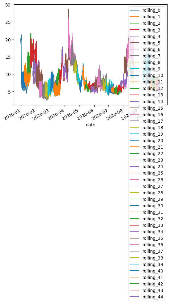
Rolling weather normalisation
[43]:
df_dewc1, mod_stats=nm.rolling(df1a, model1,feature_names=['u10', 'v10', 'd2m', 't2m',
       'blh', 'sp', 'ssrd', 'tcc', 'tp', 'rh2m','date_unix', 'day_julian', 'weekday',
       'hour'],variables_resample=['u10', 'v10', 'd2m', 't2m',
       'blh', 'sp', 'ssrd', 'tcc', 'tp', 'rh2m'], n_samples=100,window_days=14, rolling_every=7)
2024-09-24 17:12:28: Rolling window 0 from 2020-01-01 to 2020-01-14
2024-09-24 17:12:37: Rolling window 10 from 2020-03-03 to 2020-03-16
2024-09-24 17:12:47: Rolling window 20 from 2020-05-02 to 2020-05-15
2024-09-24 17:12:55: Rolling window 30 from 2020-07-01 to 2020-07-14
2024-09-24 17:13:02: Rolling window 40 from 2020-09-17 to 2020-09-30
[44]:
df_dewc1.head()
[44]:
| observed | rolling_0 | rolling_1 | rolling_2 | rolling_3 | rolling_4 | rolling_5 | rolling_6 | rolling_7 | rolling_8 | ... | rolling_35 | rolling_36 | rolling_37 | rolling_38 | rolling_39 | rolling_40 | rolling_41 | rolling_42 | rolling_43 | rolling_44 | |
|---|---|---|---|---|---|---|---|---|---|---|---|---|---|---|---|---|---|---|---|---|---|
| date | |||||||||||||||||||||
| 2020-01-01 00:00:00 | 58.1 | 20.207316 | NaN | NaN | NaN | NaN | NaN | NaN | NaN | NaN | ... | NaN | NaN | NaN | NaN | NaN | NaN | NaN | NaN | NaN | NaN |
| 2020-01-01 01:00:00 | 43.2 | 20.131948 | NaN | NaN | NaN | NaN | NaN | NaN | NaN | NaN | ... | NaN | NaN | NaN | NaN | NaN | NaN | NaN | NaN | NaN | NaN |
| 2020-01-01 02:00:00 | 43.0 | 19.247751 | NaN | NaN | NaN | NaN | NaN | NaN | NaN | NaN | ... | NaN | NaN | NaN | NaN | NaN | NaN | NaN | NaN | NaN | NaN |
| 2020-01-01 03:00:00 | 42.8 | 19.310005 | NaN | NaN | NaN | NaN | NaN | NaN | NaN | NaN | ... | NaN | NaN | NaN | NaN | NaN | NaN | NaN | NaN | NaN | NaN |
| 2020-01-01 04:00:00 | 36.8 | 20.072632 | NaN | NaN | NaN | NaN | NaN | NaN | NaN | NaN | ... | NaN | NaN | NaN | NaN | NaN | NaN | NaN | NaN | NaN | NaN |
5 rows × 46 columns
[45]:
df_dewc1.iloc[:,1:].plot()
[45]:
<Axes: xlabel='date'>
Partial Dependence Plots
[46]:
df1a=nm.prepare_data(df1, value='PM2.5', feature_names=['u10', 'v10', 'd2m', 't2m',
       'blh', 'sp', 'ssrd', 'tcc', 'tp', 'rh2m'], split_method='random',  fraction=0.75, seed=7654321)
[47]:
df1a
[47]:
| rowid | d2m | blh | ssrd | t2m | v10 | u10 | sp | tp | tcc | rh2m | date | value | date_unix | day_julian | weekday | hour | set | |
|---|---|---|---|---|---|---|---|---|---|---|---|---|---|---|---|---|---|---|
| 0 | 0 | 277.183465 | 384.209053 | -1.164153e-10 | 278.394725 | 1.545010 | -2.720528 | 102252.303312 | 0.000008 | 0.650958 | 91.884130 | 2020-01-01 00:00:00 | 58.1 | 1.577837e+09 | 1 | 3 | 0 | training |
| 1 | 1 | 276.695430 | 353.220263 | -1.164153e-10 | 277.772899 | 1.282742 | -2.308789 | 102211.168636 | 0.000002 | 0.603699 | 92.715877 | 2020-01-01 01:00:00 | 43.2 | 1.577840e+09 | 1 | 3 | 1 | training |
| 2 | 2 | 276.505662 | 255.911846 | -1.164153e-10 | 277.463419 | 0.758730 | -2.216471 | 102174.855967 | 0.000005 | 0.710378 | 93.485560 | 2020-01-01 02:00:00 | 43.0 | 1.577844e+09 | 1 | 3 | 2 | testing |
| 3 | 3 | 276.412816 | 191.375560 | -1.164153e-10 | 277.305813 | 0.509013 | -1.928623 | 102166.786485 | 0.000005 | 0.837765 | 93.906363 | 2020-01-01 03:00:00 | 42.8 | 1.577848e+09 | 1 | 3 | 3 | training |
| 4 | 4 | 276.553051 | 151.780210 | -1.164153e-10 | 277.478941 | 0.607069 | -1.700043 | 102142.578039 | 0.000003 | 0.819103 | 93.696878 | 2020-01-01 04:00:00 | 36.8 | 1.577851e+09 | 1 | 3 | 4 | testing |
| ... | ... | ... | ... | ... | ... | ... | ... | ... | ... | ... | ... | ... | ... | ... | ... | ... | ... | ... |
| 6368 | 6368 | 272.197565 | 476.945688 | -5.820766e-11 | 273.557442 | -1.945195 | 1.380939 | 99902.506413 | 0.000000 | 0.918149 | 90.582979 | 2020-12-31 19:00:00 | 11.7 | 1.609441e+09 | 366 | 4 | 19 | training |
| 6369 | 6369 | 272.171041 | 486.665851 | -5.820766e-11 | 273.629146 | -2.102732 | 0.987925 | 99947.625909 | 0.000000 | 0.839639 | 89.939908 | 2020-12-31 20:00:00 | 11.0 | 1.609445e+09 | 366 | 4 | 20 | training |
| 6370 | 6370 | 272.087408 | 489.355002 | -5.820766e-11 | 273.470592 | -1.933668 | 0.681543 | 100000.215520 | 0.000000 | 0.739354 | 90.422188 | 2020-12-31 21:00:00 | 15.3 | 1.609448e+09 | 366 | 4 | 21 | testing |
| 6371 | 6371 | 272.235319 | 40.714872 | -5.820766e-11 | 272.926062 | -0.583816 | 1.020793 | 100042.844978 | 0.000000 | 0.643753 | 95.088677 | 2020-12-31 22:00:00 | 17.1 | 1.609452e+09 | 366 | 4 | 22 | training |
| 6372 | 6372 | 272.020979 | 55.617254 | -5.820766e-11 | 272.681367 | -0.377511 | 0.959517 | 100053.601944 | 0.000000 | 0.549403 | 95.290673 | 2020-12-31 23:00:00 | 15.2 | 1.609456e+09 | 366 | 4 | 23 | training |
6373 rows × 18 columns
[49]:
all_features=['u10', 'v10', 'd2m', 't2m',
       'blh', 'sp', 'ssrd', 'tcc', 'tp', 'rh2m','date_unix', 'day_julian', 'weekday',
       'hour']
pdp_value=nm.pdp(df1a,model1,var_list=['blh'])
[50]:
pdp_value
[50]:
| variable | value | pdp_mean | pdp_std | |
|---|---|---|---|---|
| 0 | blh | 73.415911 | 15.742461 | 8.358786 |
| 1 | blh | 88.917320 | 15.359839 | 8.271418 |
| 2 | blh | 104.418730 | 14.966788 | 8.354652 |
| 3 | blh | 119.920140 | 15.582338 | 8.428540 |
| 4 | blh | 135.421549 | 13.699515 | 7.471944 |
| ... | ... | ... | ... | ... |
| 95 | blh | 1546.049822 | 6.940856 | 4.955734 |
| 96 | blh | 1561.551231 | 6.955089 | 4.957737 |
| 97 | blh | 1577.052641 | 6.960697 | 4.952725 |
| 98 | blh | 1592.554051 | 7.132266 | 4.943666 |
| 99 | blh | 1608.055460 | 7.126766 | 4.943877 |
100 rows × 4 columns
[51]:
pdp_value=nm.pdp(df1a,model1,var_list=['blh','t2m'])
[52]:
pdp_value
[52]:
| variable | value | pdp_mean | pdp_std | |
|---|---|---|---|---|
| 0 | blh | 73.415911 | 15.742461 | 8.358786 |
| 1 | blh | 88.917320 | 15.359839 | 8.271418 |
| 2 | blh | 104.418730 | 14.966788 | 8.354652 |
| 3 | blh | 119.920140 | 15.582338 | 8.428540 |
| 4 | blh | 135.421549 | 13.699515 | 7.471944 |
| ... | ... | ... | ... | ... |
| 195 | t2m | 294.518468 | 10.544835 | 7.865555 |
| 196 | t2m | 294.715875 | 10.532480 | 7.856032 |
| 197 | t2m | 294.913281 | 10.565610 | 7.847180 |
| 198 | t2m | 295.110688 | 10.527926 | 7.840150 |
| 199 | t2m | 295.308095 | 10.515571 | 7.841594 |
200 rows × 4 columns
[53]:
all_features=['u10', 'v10', 'd2m', 't2m',
       'blh', 'sp', 'ssrd', 'tcc', 'tp', 'rh2m','date_unix', 'day_julian', 'weekday',
       'hour']
pdp_value=nm.pdp(df1a,model1)
[54]:
pdp_value
[54]:
| variable | value | pdp_mean | pdp_std | |
|---|---|---|---|---|
| 0 | weekday | 1.0 | 8.808568 | 7.348096 |
| 1 | weekday | 2.0 | 8.975131 | 7.397715 |
| 2 | weekday | 3.0 | 9.519126 | 7.803357 |
| 3 | weekday | 4.0 | 9.178989 | 7.852847 |
| 4 | weekday | 5.0 | 9.756207 | 7.741670 |
| ... | ... | ... | ... | ... |
| 1226 | hour | 19.0 | 9.648269 | 7.468077 |
| 1227 | hour | 20.0 | 9.583308 | 7.474737 |
| 1228 | hour | 21.0 | 9.275591 | 7.467640 |
| 1229 | hour | 22.0 | 9.089483 | 7.493595 |
| 1230 | hour | 23.0 | 8.733808 | 7.531601 |
1231 rows × 4 columns
[ ]: